1. What is Correlation?
Correlation is a statistical technique that measures the degree and direction of relationship between two or more variables.
| Simple Definition |
| Correlation tells us: Do two things move together? Example: When temperature rises, do ice cream sales also rise? If YES → They are correlated. If NO → They are not correlated. |
Key Point: Correlation does NOT mean Causation. Just because two variables move together doesn’t mean one causes the other.
2. Types of Correlation
A. Based on Direction
| Type | Meaning | Example |
| Positive Correlation | Both variables move in the SAME direction | Height ↑ Weight ↑ |
| Negative Correlation | Variables move in OPPOSITE directions | Price ↑ Demand ↓ |
| Zero Correlation | NO relationship between variables | Shoe size & IQ |
B. Based on Number of Variables
| Type | Meaning | Example |
| Simple | 2 variables only | Price vs Demand |
| Multiple | 3 or more variables | Crop yield vs Rain, Fertilizer |
| Partial | 2 variables, effect of others removed | Income vs Savings (removing age) |
C. Based on Ratio of Change
| Type | Meaning | Graph Shape |
| Linear | Constant ratio of change | Straight line on graph |
| Non-Linear (Curvilinear) | Changing ratio | Curve on graph |
3. Methods of Studying Correlation
| Overview of Methods |
| 1. Scatter Diagram Method — Visual/Graphical 2. Karl Pearson’s Coefficient (r) — Mathematical (Quantitative data) 3. Spearman’s Rank Correlation (ρ) — Mathematical (Ranked/Qualitative data) |
4. Scatter Diagram Method
A scatter diagram is a graph where each pair of values (X, Y) is plotted as a dot. The pattern of dots shows the type and strength of correlation.
| Pattern | Type | r value |
| Dots rise left to right | Positive Correlation | +ve |
| Dots fall left to right | Negative Correlation | –ve |
| Dots scattered randomly | No Correlation | 0 |
| Dots close to a line | High Correlation | ±1 |
| Dots spread widely | Low Correlation | Near 0 |
Advantage: Quick visual understanding. Limitation: Cannot give exact numerical value of correlation.
5. Method 1: Karl Pearson’s Coefficient (r)
This is the most widely used method to calculate the exact value of correlation between two quantitative variables.
| Formula |
| r = Σ(X–X̄)(Y–Ȳ) / √[Σ(X–X̄)² × Σ(Y–Ȳ)²] OR equivalently: r = [ΣXY – n·X̄·Ȳ] / √[(ΣX² – nX̄²)(ΣY² – nȲ²)] |
Where:
- X̄ = Mean of X values
- Ȳ = Mean of Y values
- n = Number of pairs of observations
- r always lies between –1 and +1
Properties of r:
- r = +1 → Perfect positive correlation
- r = –1 → Perfect negative correlation
- r = 0 → No correlation
- r is unit-free (no units like kg, cm, etc.)
- r is not affected by change of origin or scale
6. Method 2: Spearman’s Rank Correlation (ρ)
Used when data is in the form of ranks (ordinal data) or when exact measurement is not possible.
| Formula (Without Repeated Ranks) |
| ρ = 1 – [6ΣD² / n(n²–1)] |
| Formula (With Repeated Ranks) |
| ρ = 1 – [6(ΣD² + CF) / n(n²–1)] Correction Factor (CF) = (m³–m)/12 for each tie group (m = number of tied ranks) |
Where:
- D = Difference between ranks (R₁ – R₂)
- n = Number of pairs
- ρ lies between –1 and +1
7. Solved Problems
| Solved Problem 1 — Karl Pearson’s Method |
| Find the Karl Pearson’s coefficient of correlation for the following data: |
| X | Y | XY | X² | Y² |
| 10 | 15 | 150 | 100 | 225 |
| 20 | 25 | 500 | 400 | 625 |
| 30 | 35 | 1050 | 900 | 1225 |
| 40 | 40 | 1600 | 1600 | 1600 |
| 50 | 50 | 2500 | 2500 | 2500 |
| ΣX=150 | ΣY=165 | ΣXY=5800 | ΣX²=5500 | ΣY²=6175 |
n = 5, X̄ = 150/5 = 30, Ȳ = 165/5 = 33
r = [5800 – 5×30×33] / √[(5500 – 5×900)(6175 – 5×1089)]
r = [5800 – 4950] / √[(5500–4500)(6175–5445)]
r = 850 / √[1000 × 730] = 850 / √730000 = 850 / 854.4 = 0.9948
Answer: r = 0.995 (approx.) → Very high positive correlation
| Solved Problem 2 — Spearman’s Rank Method |
| Two judges ranked 8 contestants. Find the rank correlation coefficient. |
| R₁ (Judge A) | R₂ (Judge B) | D = R₁–R₂ | D² |
| 1 | 2 | -1 | 1 |
| 2 | 1 | 1 | 1 |
| 3 | 4 | -1 | 1 |
| 4 | 3 | 1 | 1 |
| 5 | 6 | -1 | 1 |
| 6 | 5 | 1 | 1 |
| 7 | 8 | -1 | 1 |
| 8 | 7 | 1 | 1 |
| ΣD² | 8 |
ρ = 1 – [6 × 8 / 8(64–1)] = 1 – 48/504 = 1 – 0.0952 = 0.905
Answer: ρ = 0.905 → High positive correlation
| Solved Problem 3 — Karl Pearson (Larger Dataset) |
| Calculate r for the following data of advertising expenditure (X in ₹1000) and sales (Y in ₹1000): |
| X | Y | XY | X² | Y² |
| 5 | 40 | 200 | 25 | 1600 |
| 10 | 50 | 500 | 100 | 2500 |
| 15 | 60 | 900 | 225 | 3600 |
| 20 | 80 | 1600 | 400 | 6400 |
| 25 | 90 | 2250 | 625 | 8100 |
| 30 | 100 | 3000 | 900 | 10000 |
| Σ=105 | Σ=420 | Σ=8450 | Σ=2275 | Σ=32200 |
n = 6, X̄ = 17.5, Ȳ = 70
r = [8450 – 6×17.5×70] / √[(2275 – 6×306.25)(32200 – 6×4900)]
r = [8450 – 7350] / √[(2275–1837.5)(32200–29400)]
r = 1100 / √[437.5 × 2800] = 1100 / √1225000 = 1100 / 1106.8 = 0.9939
Answer: r = 0.994 → Very strong positive correlation
| Solved Problem 4 — Karl Pearson (Negative Correlation) |
| Price (X) and Demand (Y) for a commodity. Find r. |
| X (Price) | Y (Demand) | XY | X² | Y² |
| 2 | 50 | 100 | 4 | 2500 |
| 4 | 40 | 160 | 16 | 1600 |
| 6 | 35 | 210 | 36 | 1225 |
| 8 | 25 | 200 | 64 | 625 |
| 10 | 15 | 150 | 100 | 225 |
| Σ=30 | Σ=165 | Σ=820 | Σ=220 | Σ=6175 |
n = 5, X̄ = 6, Ȳ = 33
r = [820 – 5×6×33] / √[(220 – 5×36)(6175 – 5×1089)]
r = [820 – 990] / √[(220–180)(6175–5445)] = –170 / √[40×730]
r = –170 / √29200 = –170 / 170.88 = –0.9948
Answer: r = –0.995 → Very strong negative correlation
| Solved Problem 5 — Spearman’s (With Repeated Ranks) |
| Marks of 7 students in two subjects. Some marks are equal. Find ρ. |
| Student | Marks A | Rank R₁ | Marks B | Rank R₂ | D | D² |
| P | 68 | 2 | 65 | 3 | -1 | 1 |
| Q | 64 | 3.5 | 68 | 2 | 1.5 | 2.25 |
| R | 75 | 1 | 70 | 1 | 0 | 0 |
| S | 55 | 6 | 60 | 4 | 2 | 4 |
| T | 64 | 3.5 | 58 | 5 | -1.5 | 2.25 |
| U | 50 | 7 | 45 | 7 | 0 | 0 |
| V | 60 | 5 | 50 | 6 | -1 | 1 |
| ΣD² | 10.5 |
Repeated rank: 64 appears twice in A → Ranks 3 & 4 → Average = 3.5, m = 2
CF = (2³–2)/12 = 6/12 = 0.5
ρ = 1 – [6(10.5 + 0.5) / 7(49–1)] = 1 – [66/336] = 1 – 0.1964 = 0.804
Answer: ρ = 0.804 → High positive correlation
| Solved Problem 6 — Karl Pearson (Step Deviation Method) |
| Use step deviation to find r when: X: 100, 200, 300, 400, 500 and Y: 30, 50, 60, 80, 100 |
Take A = 300 (assumed mean for X), B = 60 (assumed mean for Y)
Let dX = (X–300)/100, dY = (Y–60)/10
| X | Y | dX | dY | dX×dY | dX² | dY² |
| 100 | 30 | -2 | -3 | 6 | 4 | 9 |
| 200 | 50 | -1 | -1 | 1 | 1 | 1 |
| 300 | 60 | 0 | 0 | 0 | 0 | 0 |
| 400 | 80 | 1 | 2 | 2 | 1 | 4 |
| 500 | 100 | 2 | 4 | 8 | 4 | 16 |
| Σ | 0 | 2 | 17 | 10 | 30 |
r = [ΣdXdY – n·d̄X·d̄Y] / √[(ΣdX² – nd̄X²)(ΣdY² – nd̄Y²)]
r = [17 – 5×0×0.4] / √[(10 – 0)(30 – 5×0.16)] = [17–0] / √[10 × 29.2]
r = 17 / √292 = 17 / 17.088 = 0.9948
Answer: r = 0.995 → Very strong positive correlation
Note: Step deviation simplifies calculations but gives the SAME r value!
| Solved Problem 7 — Spearman’s (Ranks Given Directly) |
| 10 students ranked by two teachers. Find ρ. |
| Student | R₁ | R₂ | D | D² |
| A | 1 | 3 | -2 | 4 |
| B | 2 | 1 | 1 | 1 |
| C | 3 | 5 | -2 | 4 |
| D | 4 | 2 | 2 | 4 |
| E | 5 | 4 | 1 | 1 |
| F | 6 | 8 | -2 | 4 |
| G | 7 | 6 | 1 | 1 |
| H | 8 | 7 | 1 | 1 |
| I | 9 | 10 | -1 | 1 |
| J | 10 | 9 | 1 | 1 |
| ΣD² | 22 |
ρ = 1 – [6×22 / 10(100–1)] = 1 – 132/990 = 1 – 0.1333 = 0.867
Answer: ρ = 0.867 → High positive agreement
| Solved Problem 8 — Perfect Positive Correlation |
| X: 1, 2, 3, 4, 5 and Y: 2, 4, 6, 8, 10. Find r. |
| X | Y | XY | X² | Y² |
| 1 | 2 | 2 | 1 | 4 |
| 2 | 4 | 8 | 4 | 16 |
| 3 | 6 | 18 | 9 | 36 |
| 4 | 8 | 32 | 16 | 64 |
| 5 | 10 | 50 | 25 | 100 |
| Σ=15 | Σ=30 | Σ=110 | Σ=55 | Σ=220 |
r = [110 – 5×3×6] / √[(55–45)(220–180)] = 20/√[10×40] = 20/20 = 1.00
✅ Answer: r = +1.00 → Perfect positive correlation (Y = 2X)
| Solved Problem 9 — Karl Pearson (Real-World: Study Hours vs Marks) |
| Hours studied (X) and Marks obtained (Y). Find r. |
| X (Hours) | Y (Marks) | XY | X² | Y² |
| 2 | 40 | 80 | 4 | 1600 |
| 3 | 50 | 150 | 9 | 2500 |
| 5 | 65 | 325 | 25 | 4225 |
| 7 | 80 | 560 | 49 | 6400 |
| 8 | 85 | 680 | 64 | 7225 |
| 10 | 95 | 950 | 100 | 9025 |
| Σ=35 | Σ=415 | Σ=2745 | Σ=251 | Σ=30975 |
n = 6, X̄ = 35/6 = 5.833, Ȳ = 415/6 = 69.167
r = [2745 – 6(5.833)(69.167)] / √[(251 – 6×34.03)(30975 – 6×4784.08)]
r = [2745 – 2420.83] / √[(251–204.17)(30975–28704.5)]
r = 324.17 / √[46.83 × 2270.5] = 324.17 / √106336 = 324.17 / 326.1 = 0.9941
Answer: r = 0.994 → More study hours = Better marks!
| Solved Problem 10 — Spearman’s (Negative Correlation) |
| Ranks of 6 items by Quality (R₁) and Price (R₂). Find ρ. |
| Item | R₁ (Quality) | R₂ (Price) | D | D² |
| A | 1 | 6 | -5 | 25 |
| B | 2 | 5 | -3 | 9 |
| C | 3 | 4 | -1 | 1 |
| D | 4 | 3 | 1 | 1 |
| E | 5 | 2 | 3 | 9 |
| F | 6 | 1 | 5 | 25 |
| ΣD² | 70 |
ρ = 1 – [6×70 / 6(36–1)] = 1 – 420/210 = 1 – 2 = –1.00
✅ Answer: ρ = –1.00 → Perfect negative correlation (ranks are exactly reversed!)
8. Interpretation of r and ρ Values
| Value of r/ρ | Degree | Meaning |
| +1.00 | Perfect Positive | Variables move exactly together |
| +0.75 to +0.99 | High Positive | Strong direct relationship |
| +0.50 to +0.74 | Moderate Positive | Fair direct relationship |
| +0.25 to +0.49 | Low Positive | Weak direct relationship |
| 0 | No Correlation | No linear relationship |
| –0.25 to –0.49 | Low Negative | Weak inverse relationship |
| –0.50 to –0.74 | Moderate Negative | Fair inverse relationship |
| –0.75 to –0.99 | High Negative | Strong inverse relationship |
| –1.00 | Perfect Negative | Variables move exactly opposite |
| Important Warning |
| Correlation ≠ Causation! Example: Ice cream sales and drowning deaths are positively correlated. Does ice cream cause drowning? NO! Both increase in summer (hidden variable: temperature). Always look for the LURKING VARIABLE before concluding causation. |
9. Which Method to Use When?
| Situation | Best Method | Symbol |
| Data is quantitative (numbers) | Karl Pearson | r |
| Data is already ranked | Spearman | ρ |
| Data is qualitative (beauty, intelligence) | Spearman | ρ |
| Quick visual check needed | Scatter Diagram | Visual |
| Small sample + ordinal data | Spearman | ρ |
| Large sample + continuous data | Karl Pearson | r |
| Data has extreme outliers | Spearman (more robust) | ρ |
| Exact numerical value needed | Karl Pearson/Spearman | r or ρ |
10. Practice Problems (Try Yourself!)
| Practice 1 |
| Find Karl Pearson’s r: X: 12, 14, 16, 18, 20, 22 and Y: 25, 30, 28, 35, 40, 38 Hint: n = 6. First find ΣX, ΣY, ΣXY, ΣX², ΣY² |
| Practice 2 |
| Find Spearman’s ρ for ranks: R₁: 1,2,3,4,5,6,7 and R₂: 7,5,3,4,1,2,6 Hint: Compute D = R₁ – R₂, then ΣD² |
| Practice 3 |
| X: 5, 8, 12, 15, 18, 22, 25 and Y: 110, 95, 80, 70, 55, 40, 25. Find r and interpret. Hint: Expect a negative value! |
| Practice 4 |
| Two interviewers rank 8 candidates. Some candidates score equal marks. Find ρ with correction factor. Marks A: 75, 80, 68, 80, 90, 65, 72, 85 | Marks B: 70, 85, 65, 75, 95, 60, 70, 80 |
11. Exam Tips
| Top Exam Tips |
| Always check: –1 ≤ r ≤ +1. If your answer is outside this range, recheck!Write the formula first, then substitute values — it earns marks even if calculation goes wrong.Make a table for calculations — it’s organized and reduces errors.Don’t forget the correction factor for repeated ranks in Spearman’s!Always state interpretation: “high positive”, “moderate negative” etc.Remember: r is unit-free. Don’t write units in your answer.For step deviation method: r doesn’t change with change of origin/scale.If question asks “comment on relationship” — always mention direction + strength.Practice at least 3 problems of each type before exams.In MCQs: If all ranks are reversed, ρ = –1. If ranks are identical, ρ = +1. |
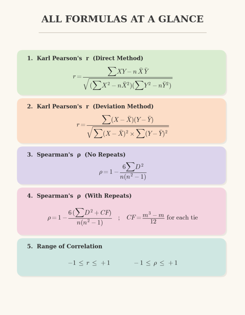
12. Formula Summary Box 📋
Swathika B is an MBA graduate in Finance & Business Analytics , the founder of The Commerce Lab. With a strong academic foundation in B.Com BFSI and hands-on experience in financial analysis, data analytics, and business studies, she created this platform to make Commerce and Accountancy simple, practical, and exam-ready for students across India.