With Step-by-Step Solved Problems & Boxed Formulas
1. Introduction — What is Standard Deviation?
In statistics, we often want to know not just the average of a set of values, but also how spread out those values are. A class where all students score 70 is very different from a class where scores range from 20 to 100 — even though both may have the same average!
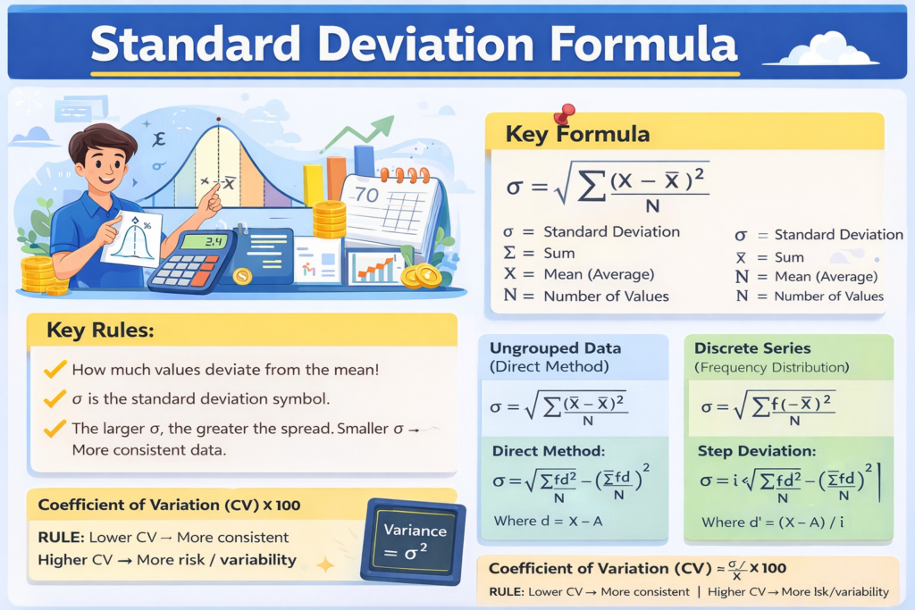
Standard Deviation (SD or σ) measures the degree of dispersion or spread of data values around the mean. The larger the SD, the more spread out the data. The smaller the SD, the more consistent or clustered the data.
| σ (sigma) = Standard Deviation Variance = σ² |
1.1 Why Standard Deviation?
| Measure | What it tells you | Limitation |
| Range | Max − Min | Affected by outliers |
| Mean Deviation | Average absolute deviation | Ignores algebraic signs |
| Standard Deviation | True spread around mean | Slightly complex to compute |
| Variance | SD squared | Not in same unit as data |
Standard Deviation is the MOST WIDELY USED measure of dispersion in statistics, economics, finance, and research because it uses ALL data values and is mathematically tractable.
2. Formulas — All Methods
2.1 For Ungrouped Data (Individual Series)
Method 1 — Direct Method:
| σ = √[ Σ(X − X̄)² / N ] Where: X = each value, X̄ = Mean, N = number of observations |
Method 2 — Shortcut / Assumed Mean Method:
| σ = √[ Σd²/N − (Σd/N)² ] Where: d = X − A (A = Assumed Mean) |
Method 3 — Direct Formula (Alternate):
| σ = √[ ΣX²/N − (X̄)² ] |
2.2 For Discrete Series (Frequency Distribution)
Direct Method:
| σ = √[ Σf(X − X̄)² / N ] |
Shortcut Method:
| σ = √[ Σfd²/N − (Σfd/N)² ] where d = X − A |
Step Deviation Method:
| σ = i × √[ Σfd′²/N − (Σfd′/N)² ] where d′ = (X − A) / i |
2.3 For Continuous Series (Class Intervals)
| σ = i × √[ Σfd′²/N − (Σfd′/N)² ] where mid-values are used as X, N = Σf |
2.4 Coefficient of Variation (CV)
| CV = (σ / X̄) × 100 Lower CV → More consistent | Higher CV → More variable |
3. Solved Problems — Individual Series
Problem 1 — Direct Method (Beginner)
Find the Standard Deviation of: 4, 8, 6, 5, 3, 2, 8, 9, 2, 5
Step 1: Find the Mean
| X̄ = (4+8+6+5+3+2+8+9+2+5) / 10 = 52 / 10 = 5.2 |
Step 2: Calculate deviations and squared deviations
| X | X − X̄ | (X − X̄)² |
| 4 | −1.2 | 1.44 |
| 8 | 2.8 | 7.84 |
| 6 | 0.8 | 0.64 |
| 5 | −0.2 | 0.04 |
| 3 | −2.2 | 4.84 |
| 2 | −3.2 | 10.24 |
| 8 | 2.8 | 7.84 |
| 9 | 3.8 | 14.44 |
| 2 | −3.2 | 10.24 |
| 5 | −0.2 | 0.04 |
| ΣX = 52 | Σ(X−X̄) = 0 | Σ(X−X̄)² = 57.60 |
Step 3: Apply the formula
| σ = √(Σ(X−X̄)² / N) = √(57.60 / 10) = √5.76 |
| σ = 2.4 |
Problem 2 — Shortcut / Assumed Mean Method (Beginner)
Find SD of: 10, 20, 30, 40, 50 using Assumed Mean A = 30
Step 1: Compute deviations d = X − A
| X | d = X − 30 | d² |
| 10 | −20 | 400 |
| 20 | −10 | 100 |
| 30 | 0 | 0 |
| 40 | 10 | 100 |
| 50 | 20 | 400 |
| N = 5 | Σd = 0 | Σd² = 1000 |
Step 2: Apply the shortcut formula
| σ = √[ Σd²/N − (Σd/N)² ] = √[ 1000/5 − (0/5)² ] = √[ 200 − 0 ] = √200 |
| σ ≈ 14.14 |
4. Solved Problems — Discrete Series
Problem 3 — Discrete, Shortcut Method (Intermediate)
Calculate Standard Deviation from the following data (A = 25):
Step 1: Prepare the table with deviations
| X | f | d = X−25 | d² | fd | fd² |
| 10 | 3 | −15 | 225 | −45 | 675 |
| 15 | 7 | −10 | 100 | −70 | 700 |
| 20 | 10 | −5 | 25 | −50 | 250 |
| 25 | 12 | 0 | 0 | 0 | 0 |
| 30 | 8 | 5 | 25 | 40 | 200 |
| 35 | 6 | 10 | 100 | 60 | 600 |
| 40 | 4 | 15 | 225 | 60 | 900 |
| — | N=50 | — | — | Σfd=−5 | Σfd²=3325 |
Step 2: Apply the shortcut formula
| σ = √[ Σfd²/N − (Σfd/N)² ] = √[ 3325/50 − (−5/50)² ] = √[ 66.5 − 0.01 ] = √66.49 |
| σ ≈ 8.15 |
5. Solved Problems — Continuous Series
Problem 4 — Class Intervals, Step Deviation (Intermediate)
Find SD using Step Deviation Method (i = 10, A = 35):
Step 1: Compute mid-values and step deviations
| Class | f | Mid (m) | d=m−35 | d′=d/10 | fd′ | fd′² |
| 5−15 | 4 | 10 | −25 | −2.5 | −10 | 25 |
| 15−25 | 8 | 20 | −15 | −1.5 | −12 | 18 |
| 25−35 | 15 | 30 | −5 | −0.5 | −7.5 | 3.75 |
| 35−45 | 20 | 40 | 5 | 0.5 | 10 | 5 |
| 45−55 | 12 | 50 | 15 | 1.5 | 18 | 27 |
| 55−65 | 6 | 60 | 25 | 2.5 | 15 | 37.5 |
| — | N=65 | — | — | — | Σfd′=13.5 | Σfd′²=116.25 |
Step 2: Apply the step deviation formula
| σ = i × √[ Σfd′²/N − (Σfd′/N)² ] = 10 × √[ 116.25/65 − (13.5/65)² ] = 10 × √[ 1.788 − 0.043 ] = 10 × √1.745 = 10 × 1.321 |
| σ ≈ 13.21 |
6. Advanced Problems
Problem 5 — Combined Standard Deviation
Two groups have the following data. Find the combined SD:
| Group A | Group B | |
| Number (n) | 40 | 60 |
| Mean (X̄) | 30 | 40 |
| Std Deviation (σ) | 8 | 10 |
Step 1: Find Combined Mean
| X̄₁₂ = (n₁X̄₁ + n₂X̄₂) / (n₁ + n₂) = (40×30 + 60×40) / (40+60) = (1200+2400)/100 = 3600/100 |
| Combined Mean = 36 |
Step 2: Compute d₁ and d₂
| d₁ = X̄₁ − X̄₁₂ = 30 − 36 = −6 d₂ = X̄₂ − X̄₁₂ = 40 − 36 = 4 |
Step 3: Apply Combined SD Formula
| σ₁₂ = √[ (n₁(σ₁²+d₁²) + n₂(σ₂²+d₂²)) / (n₁+n₂) ] = √[ (40(64+36) + 60(100+16)) / 100 ] = √[ (4000 + 6960) / 100 ] = √109.6 |
| Combined SD ≈ 10.47 |
Problem 6 — Coefficient of Variation (CV)
A factory has two machines. Compare their consistency:
| Machine A | Machine B | |
| Mean Output (units) | 200 | 250 |
| Standard Deviation | 16 | 25 |
Step 1: Calculate CV for each machine
| CV = (σ / X̄) × 100 CV of Machine A = (16 / 200) × 100 = 8% CV of Machine B = (25 / 250) × 100 = 10% |
| Machine A is MORE CONSISTENT (Lower CV = 8% < 10%) |
Problem 7 — Missing Frequency + SD (Pro Level)
In the following distribution, mean = 32 and total N = 100. Find the missing frequencies and then compute SD:
| Wages (₹) | Frequency (f) | Mid (m) |
| 10−20 | 12 | 15 |
| 20−30 | f₁ | 25 |
| 30−40 | f₂ | 35 |
| 40−50 | 20 | 45 |
| 50−60 | 8 | 55 |
Step 1: Set up frequency equation
| 12 + f₁ + f₂ + 20 + 8 = 100 f₁ + f₂ = 60 … (Equation 1) |
Step 2: Set up mean equation (mean = 32)
| Σfm / N = 32 (12×15 + f₁×25 + f₂×35 + 20×45 + 8×55) / 100 = 32 1520 + 25f₁ + 35f₂ = 3200 25f₁ + 35f₂ = 1680 … (Equation 2) |
Step 3: Solve simultaneous equations
| From Eq.1: f₁ = 60 − f₂ 25(60 − f₂) + 35f₂ = 1680 1500 − 25f₂ + 35f₂ = 1680 10f₂ = 180 → f₂ = 18, f₁ = 42 |
| f₁ = 42, f₂ = 18 |
Step 4: Compute SD using Step Deviation (A = 35, i = 10)
| Class | f | m | d=m−35 | d′=d/10 | fd′ | fd′² |
| 10−20 | 12 | 15 | −20 | −2 | −24 | 48 |
| 20−30 | 42 | 25 | −10 | −1 | −42 | 42 |
| 30−40 | 18 | 35 | 0 | 0 | 0 | 0 |
| 40−50 | 20 | 45 | 10 | 1 | 20 | 20 |
| 50−60 | 8 | 55 | 20 | 2 | 16 | 32 |
| — | 100 | — | — | — | Σfd′=−30 | Σfd′²=142 |
Step 5: Apply formula
| σ = 10 × √[ 142/100 − (−30/100)² ] = 10 × √[ 1.42 − 0.09 ] = 10 × √1.33 = 10 × 1.153 |
| σ ≈ 11.53 |
7. Key Properties of Standard Deviation
• It is always non-negative (σ ≥ 0). SD = 0 means all values are identical.
• It is expressed in the SAME UNITS as the original data.
• Adding/subtracting a constant to all values does NOT change σ.
• Multiplying all values by a constant k multiplies σ by |k|.
• Among all measures of dispersion, SD is least affected by sampling fluctuations.
• SD is used in computing CV, Pearson’s Coefficient, and Normal Distribution.
7.1 Empirical Rule (Normal Distribution)
| Range | % of data covered | Rule |
| X̄ ± 1σ | 68.27% | ~68% Rule |
| X̄ ± 2σ | 95.45% | ~95% Rule |
| X̄ ± 3σ | 99.73% | ~99.7% Rule |
8. Comparison — All Dispersion Measures
| Feature | Range | Mean Dev. | SD | Variance |
| Uses all values? | No | Yes | Yes | Yes |
| Algebraic signs? | N/A | Ignored | Squared | Squared |
| Same unit as data? | Yes | Yes | Yes | No |
| Best for inference? | No | No | Yes | No |
9. Formula Quick Reference
Individual (Direct):
| σ = √[Σ(X−X̄)² / N] |
Individual (Shortcut):
| σ = √[Σd²/N − (Σd/N)²] |
Discrete (Shortcut):
| σ = √[Σfd²/N − (Σfd/N)²] |
Step Deviation:
| σ = i×√[Σfd′²/N − (Σfd′/N)²] |
Coefficient of Variation: CV = (σ/X̄) × 100
| CV = (σ/X̄) × 100 |
Combined SD:
| σ₁₂ = √[(n₁(σ₁²+d₁²)+n₂(σ₂²+d₂²))/(n₁+n₂)] |
10. Exam Strategy & Common Mistakes
| Common Mistake | Correct Approach |
| Using mid-values wrong in CI | Always compute m = (Lower + Upper) / 2 |
| Forgetting to square d in Σd² | Double check: fd² column vs fd column |
| Wrong N (using n of X not Σf) | N = Σf for grouped data always |
| Not multiplying by i at end | Step deviation always needs × i final step |
Swathika B is an MBA graduate in Finance & Business Analytics , the founder of The Commerce Lab. With a strong academic foundation in B.Com BFSI and hands-on experience in financial analysis, data analytics, and business studies, she created this platform to make Commerce and Accountancy simple, practical, and exam-ready for students across India.